
klrfome - Kernel Logistic Regression on Focal Mean Embeddings
The purpose of this package is to solve the Distribution Regression problem for archaeological site location modeling; or any other data for that matter. The aim of Distribution Regression is to map a single scalar outcome (e.g. presence/absence; 0/1) to a distribution of features. This is opposed to typical regression where you have one observation mapping a single outcome to a single set of features/predictors. For example, an archaeological site is singularly defined as either present or absent, however the area within the sites boundary is not singularly defined by any one measurement. The area with an archaeology site is defined by an infinite distribution of measurements. Modeling this in traditional terms means either collapsing that distribution to a single measurement or pretending that a site is actually a series of adjacent, but independent measurements. The methods developed for this package take a different view instead by modeling the distribution of measurements from within a single site on a scale of similarity to the distribution of measurements on other sites and the environmental background in general. This method avoids collapsing measurements and promotes the assumption of independence from within a site to between sites. By doing so, this approach models a richer description of the landscape in a more intuitive sense of similarity.
To achieve this goal, the package fits a Kernel Logistic Regression (KLR) model onto a mean embedding similarity matrix and predicts as a roving focal function of varying window size. The name of the package is derived from this approach; Kernel Logistic Regression on FOcal Mean Embeddings (klrfome) pronounced clear foam.

(High-res versions of research poster are in the /SAA_2018_poster folder)
Citation
Please cite this package as:
Harris, Matthew D., (2017). klrfome - Kernel Logistic Regression on Focal Mean Embeddings. Accessed 10 Sep 2017. Online at https://doi.org/10.5281/zenodo.1218403
Special Thanks
This model is inspired by and borrows from Zoltán Szabó’s work on mean embeddings (Szabó et al. 2016, @Szabo2) and Ji Zhu & Trevor Hastie’s Kernel Logistic Regression algorithm (Zhu and Hastie 2005). I extend a hardy thank you to Zoltán for his correspondence during the development of this approach. This approach would not have been created without his help. Further, a big thank you to Ben Markwick for his moral support and rrtools package used to create this package. However that being said, all errors, oversights, and omissions are my own.
Installation
You can install klrfome from github with:
Example workflow on simulated data (Try me!)
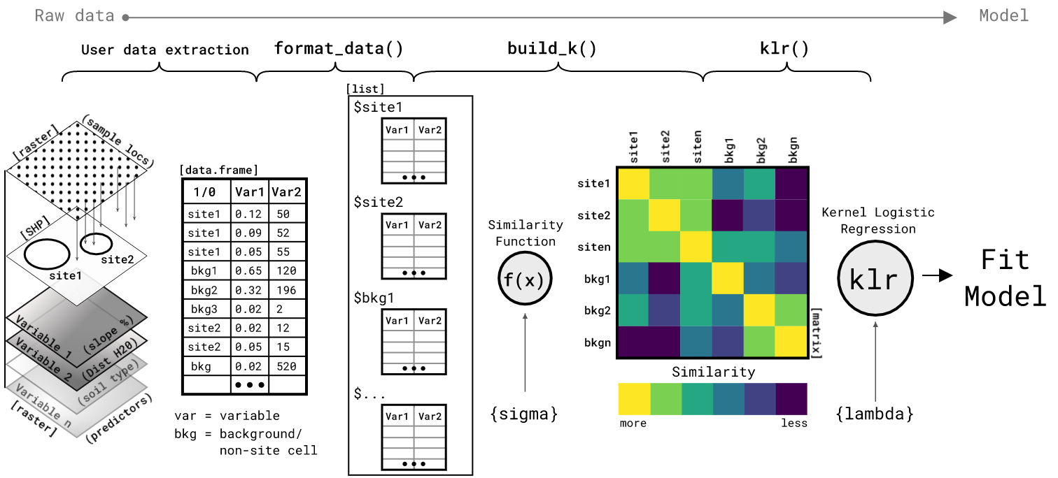
In brief, the process below is 1) take a table of observations of two or more environmental variables within known sites and across the background of the study area; 2) use format_data() to convert that table to a list and under-sample the background data to a desired ratio (each group of observations with a site or background area are referred o in the ML literature as “bags”); 3) use build_k() function with the sigma hyperparameter and distance (default euclidean) to create a similarity matrix between all site and background bags; 4) the similarity matrix is the object that the kernel logistic regression model klr() function uses to fit its parameters. Steps 3 and 4 are where this method detracts most from traditional regression, but it is also what sets this method apart. unlike most regression that fits a model to a table of measurements, this approach fits a model to a matrix of similarities between all of the units of analysis (sites and background areas).
Set hyperparameters and load simulated site location data
In this block, the random seed, sigma and lambda hyperparameters, and the dist_metric are all set. The sigma parameter controls how “close” observations must be to be considered similar. Closeness in this context is defined in the ‘feature space’, but in geographic or measurement space. At a higher sigma more distant observations can still be considered similar. The lambda hyperparameter controls the regularization in the KLR model by penalizing large coefficients; it must by greater than zero. This means that the higher the lambda penalty, the closer the model will shrink its alpha parameters closer to zero, thereby reducing the influence of any one or group of observations on the overall model. These two hyperparameters are most critical as the govern the flexibility and scope of the model. Ideally, these will be set via k-fold Cross-Validation, Leave-one-out cross-validation, grid search, or trial and error. Exploring these hyperparameters will likely take most of the time and attention within the modeling process.
Build Similarilty kernel, fit KLR model, and predict on training set
The first step in modeling these data is to build the similarity kernel with build_k. The output is a pairwise similarity matrix for each element of the list you give it, in this case training_data. The object K is the NxN similarity matrix of the mean similarity between the multivariate distance of each site and background list element. These elements are often referred to as laballed bags because they are a collection of measurements with a presence or absence label. The second step is to fit the KLR model with the KLR function. The KLR fit function is a key component of this package. The function fits a KLR model using Iterative Re-weighted Least Squares (IRLS). Verbose = 2 shows the convergence of the algorithm. The output of this function is a list of the alpha parameters (for prediction) and predicted probability of site-present for the train_data set. Finally, the KLR_predict function uses the train_data and alphas to predict the probability of site-presence for new test_data. The similarity matrix can be visualized with corrplot, the predicted site-presence probability for simulated site-present and background test data can be viewed as a ggplot, and finally the parameters of the model are saved to a list to be used for predicting on a study area raster stack.


Predicting on a raster stack
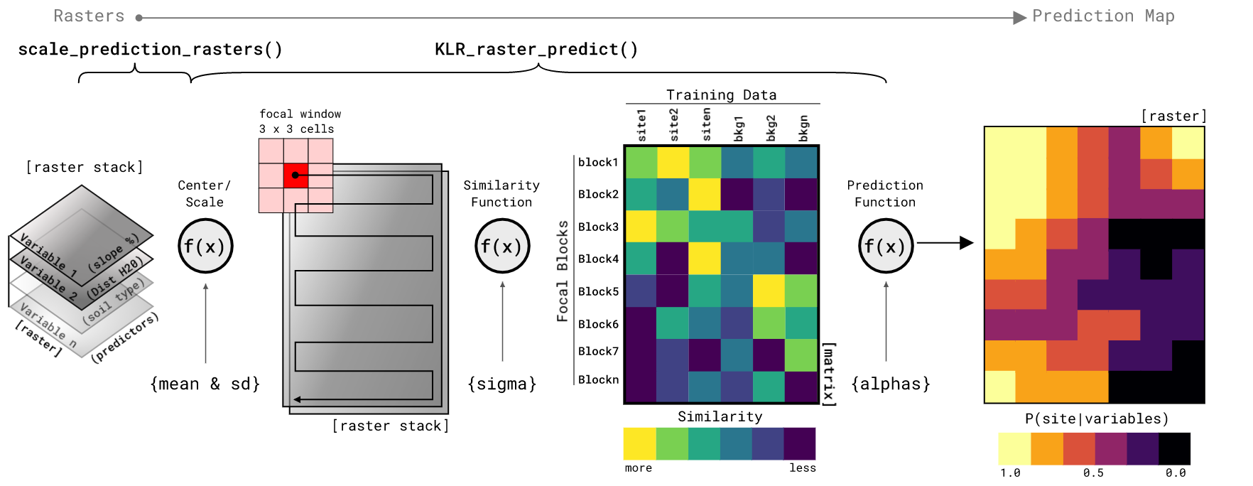
This package can be used to predict on tabular data as above, but a more practical approach is to predict directly on a set of raster layers representing the predictor variables. Most of the code below is there for creating a simulated landscape that has some fidelity to the training data. For real-world examples, the prediction starts with a raster stack of predictor variable rasters. Form there the function scale_prediction_rasters center and scales the values of the rasters to that of the train_data. Having data that is centered at zero and scaled to z-scores is critical in measuring the distance between observations. Further, it is critical that the test data (raster stack) is scaled to the same values as the training data or the predictions will be invalid. Once scaled, the raster stack is sent to the KLR_raster_predict function for prediction. The prediction function requires a scaled raster stack of the same variables used to train the model, the ngb value that specifies the x and y dimension of the focal window, and finally the list of params from the trained model. The setting on KLR_raster_predict shown here are predicting over the entire raster at once and not in parallel. The KLR_raster_predict function has options for splitting the prediction into a number of squares and predicting on each of those. Further, each split raster block can be assigned to a different core on your computer to compute in parallel. This is because prediction is a time consuming process and it is often helpful to split the computation into more manageable blocks. Oh, and you can set it to return the predicted blocks as a list of raster (all in memory) or to save each block as a GeoTiff after it is predicted. A version of parallel processing is shown in the next code section.

Predicting in parallel/multi-core
This package uses the foreach package’s %dopar% function to parallelize model prediction. To make this work you need to start a parallel backend. Here I show how to do this with doParallel package. It is simple in most cases, just make a cluster with makeCluster and the number of cores you have available and then register the cluster with registerDoParallel (note the use of stopCluster() when you are done). In the KLR_raster_predict function, you need to set a few things. Set parallel = TRUE, split = TRUE, and ppside is the number of raster blocks on the x and y axis (resulting in ppside^2 number of output rasters). The function also gives the options for output = "list" to return a list or output = "save" to save each raster as a GeoTiff to the save_loc directory. Finally, the cols and rows values are used here so that the split function knows the dimensions of the entire prediction raster. It need to know this becuase it mitigates the edge effect predicting on blocks by putting a collar of size ngb around each block. The cols and rows lets the function know when to remove the collar and when it is at an edge of the study area.

Model Evaluation
Evaluating model on independent test data is very important for understanding the models ability to generalize to new observations. The klrfome package provides two functions to assist with this; CM-quads() and metrics(). In order to use these functions, the user needs to extract the sensitivity values output from klr_raster_predict at both site locations (preferably not those used to create the model) and a large number of random locations to sample the full distribution of sensitivities. The code below uses the simulated site locations, raster::extract, and sampleRandom to obtain these values. Once the values are put into a table and labelled as 1 or 0, the CM-quads function is applied to retrieve the True Positive, True Negative, False Positive, and False Negative values of the model at one or more probability thresholds. Choosing the appropriate threshold at which to classify a model into High, Moderate, and Low or Site-present vs. site-absent needs a good deal of consideration for both the intrinsic model quality and extrinsic model goals. Here I show how to evaluate the classification metrics at every 0.1 threshold between 0 and 1. The results from CM_quads (named for the four quadrants of the confusion matrix) are then evaluated with the pROC::auc and klrfome::metrics functions to calculate the metrics of choice.
| 0.0 |
336 |
500 |
0 |
0 |
0.85 |
0.000 |
0.000 |
1.000 |
1.000 |
0.000 |
| 0.1 |
336 |
357 |
143 |
0 |
0.85 |
0.286 |
0.286 |
1.000 |
0.714 |
0.000 |
| 0.2 |
334 |
281 |
219 |
2 |
0.85 |
0.432 |
0.435 |
0.994 |
0.562 |
0.006 |
| 0.3 |
322 |
237 |
263 |
14 |
0.85 |
0.484 |
0.505 |
0.958 |
0.474 |
0.042 |
| 0.4 |
318 |
203 |
297 |
18 |
0.85 |
0.540 |
0.571 |
0.946 |
0.406 |
0.054 |
| 0.5 |
311 |
179 |
321 |
25 |
0.85 |
0.568 |
0.613 |
0.926 |
0.358 |
0.074 |
| 0.6 |
296 |
150 |
350 |
40 |
0.85 |
0.581 |
0.659 |
0.881 |
0.300 |
0.119 |
| 0.7 |
277 |
126 |
374 |
59 |
0.85 |
0.572 |
0.694 |
0.824 |
0.252 |
0.176 |
| 0.8 |
238 |
96 |
404 |
98 |
0.85 |
0.516 |
0.729 |
0.708 |
0.192 |
0.292 |
| 0.9 |
112 |
42 |
458 |
224 |
0.85 |
0.249 |
0.748 |
0.333 |
0.084 |
0.667 |
| 1.0 |
0 |
0 |
500 |
336 |
0.85 |
0.000 |
NaN |
0.000 |
0.000 |
1.000 |
In this case those metrics are the auc, Youdens J, KG = Kvamme Gain, Sensitivity, FPR = False Positive Rate, and FNR = False Negative Rate. While there is no one metric that is a perfect descriptor of model performance in all scenarios, these are the metrics that I find most useful for describing archaeological predictive models. In this example, I am aiming to maximize my two-class classification for the Youden’s J (aka Informedness). As such, I would set my site-present vs. site-absent Threshold at 0.6. At this threshold we have a Sensitivity = 0.881 and a FPR = 0.3.
Main Package Functions
This package contains the functions necessary to compute Kernel Linear Regression (KLR) on mean kernel embeddings, functions for preparing site and background data, and a function for simulate archaeological site location data.
KLR_funs.R for Fitting and Predicting on Tabular Data
build_K - Function takes list of training data, scalar value for sigma hyperparameter, and a distance method to compute a mean embedding similarity kernel. This kernel is a pair-wise (N x N) matrix of the mean similarity between the attributes describing each site location and background group. Optional inouts are progress for a progress bar and dist_metric for the distance computation. By default, the distance metric is euclidean and should likely stay as such unless you have explored other distances and know why/how you want to use them.
KLR - Function takes the similarity kernel matrix K, a vector of presence/absence coded as 1 or 0, and a scalar value for the lambda regularizing hyperparameter; optionally values for maximum iterations and threshold. This function performs Kernel Logistic Regression (KLR) via Iterative Re-weighted Least Squares (IRLS). The objective is to approximate a set of parameters that minimize the negative likelihood of the parameters given the data and response. This function returns a list of pred, the estimated response (probability of site-presence) for the training data, and alphas, the approximated parameters from the IRLS algorithm.
KLR_predict - Function takes a list of the training data, a list of the testing data, a vector of the approximated alphas parameters, a scalar value for the sigma kernel hyperparameter, and a distance method. This function predicts the probability of site presence for new observations based on the training data and alphas parameters. This is accomplished by building the k*k kernel matrix as the similarity between the training test data then computing the inverse logit of k*k %*% alphas. The output is the predicted probability of site presence for each training data example.
raster_predict_funs.R for Predicting on Raster Data
rescale_sim_raster - Function that rescales simulated rasters from NLMR::nlm_gaussianfield (Sciaini, Fritsch, and Simpkins 2017) or whatever you want to use, to the mean and standard deviation of the simulated data used to fit the klr model. You will have to add the mean and sd arguments manually based on what you put into the get_sim_data function. The example in the code above inputs the default mean and sd values from the defualts of the get_sim_data function. Returned is a raster scaled too your simualted training data.
sim_trend - Function is used to take create n number of simulated site locations of size cell dimensions on a rows by cols raster. The latter two arguments should match the size of your simulated rasters. The function randomly locates the sites and then creates a distance gradient (trend) from the site locations outward. The trend is a value 1 at the sites and reduces to 0 at the maximum combined distance from all sites. The output of this function is a list of a matrix of simulated site x/y coordinates (centers) and a raster of the trend surface. The point of the trend is to then combine it with the simulated rasters (as down in the code above) such that the raster depicting site-likely conditions is multiplied by the trend to output a raster retaining site-likely conditions near simulated site locations. Conversely, the site-unlikely simulated raster is multiplied by the inverse of the trend to result in a raster retaining site-unlikely characteristics away from the site locations. When those two rasters are added you get a simulated environment that is more preferable to site locations near site locations. It is a bit involved for something that had nothing to do with the actual KLRfome model, but it is needed to produce actual correlated environments for model testing.
scale_prediction_rasters - Function scales your predictor rater stack based on the params list created in the model fitting process. This script simply loops over the rasters in the stack and centers and scales based on mean and sd of the training data used to fit the klr model. The function outputs a raster stack.
KLR_raster_predict - Function predicts the probability of site-presence based on a raster stack of center/scaled predictor rasters, a focal neighborhood size in cells as ngb, and the params list of model fit parameters. Finally, the function also needs to the the number of columns as cols and rows as rows of the study areas raster stack. The rest of the arguments default to predicting the entire raster stack in one pass and only on a single core (not in parallel). The rest of the argument control whether the study area is split (split = TRUE) into a grid of blocks. The ppside positive integer controls the number of blocks along each axis of the study area. If you wish to compute the prediction in parallel, you will need to split it into blocks so that each block can be sent to a different processor core. The final set of optional arguments control how the prediction is returned, either as a output = "list" or output = "save" for returning a list of rasters of saving each out as a GeoTiff, and then arguments for the GeoTiff location with save_loc and whether to overwrite existing GeoTiffs with overwrite. The function contains a bit of logic to try and assist the user in which arguments go with what. Perhaps future versions will streamline this a bit.
get_sim_data.R for Simulating Site Location Data
-
get_sim_data - Function takes a mean and SD for two simulated predictor variables for each of sites and background. With archaeological site data being a protected data set in many settings (including this project), it cannot be freely shared. However, it is difficult to implement this model without properly format data. This function simulates archaeological site data and background environmental data for testing or tuning of this model. The concept of the function is to simulate two predictor variables for both sites and background. The inputs to the function (defaults provided) control how similar or different the site data is from the background. The model can be tested on simulated site data that is very similar to the background or very different; the model behaves accordingly. The output of the function is formatted in the same way as the format_site_data function.
plot.R for Plotting Similarity Kernel
-
K_corrplot - Function is a pretty simple wrapper around corrplot::corrplot() with hierarchical clustering. Inputs for this function are the similarity matrix K and the train_data with the option of an integer for the number of clusters to partition the data; default = 4. Output is a plot or if assigned to an object, it is an object of class matrix.
Contributions
We welcome contributions from everyone. Before you get started, please see our contributor guidelines. Please note that this project is released with a Contributor Code of Conduct. By participating in this project you agree to abide by its terms.
References
Flaxman, Seth, Yu-Xiang Wang, and Alexander J. Smola. 2015. “Who Supported Obama in 2012?: Ecological Inference Through Distribution Regression.” In Proceedings of the 21th Acm Sigkdd International Conference on Knowledge Discovery and Data Mining, 289–98. ACM.
Law, H. C. L., D. J. Sutherland, D. Sejdinovic, and S. Flaxman. 2017. “Bayesian Approaches to Distribution Regression.” ArXiv E-Prints, May. http://arxiv.org/abs/1705.04293.
Muandet, Krikamol, Kenji Fukumizu, Bharath Sriperumbudur, and Bernhard Schölkopf. 2017. “Kernel Mean Embedding of Distributions: A Review and Beyond.” Foundations and Trends in Machine Learning 10 (1-2): 1–141. https://doi.org/10.1561/2200000060.
Song, Li, and Arthur Fukumizu Kenjiand Gretto. 2013. “Kernel Embeddings of Conditional Distributions: A Unified Kernel Framework for Nonparametric Inference in Graphical Models.” IEEE Signal Processing Magazine 30 (4): 98–111. https://doi.org/10.1109/msp.2013.2252713.
Szabó, Zoltán, Arthur Gretton, Barnabás Póczos, and Bharath Sriperumbudur. 2015. “Two-Stage Sampled Learning Theory on Distributions.” In International Conference on Artificial Intelligence and Statistics (Aistats), 948–57.
Szabó, Zoltán, Bharath Sriperumbudur, Barnabás Póczos, and Arthur Gretton. 2016. “Learning Theory for Distribution Regression.” Journal of Machine Learning Research 17: 1–40.
Zhu, Ji, and Trevor Hastie. 2005. “Kernel Logistic Regression and the Import-Vector Machine.” Journal of Computational and Graphical Statistics 14 (1): 185–205. https://doi.org/10.1198/106186005x25619.
